Non-parametric matched pair testing with left-censored data

Comparing two groups of measurements when some values are below one or multiple detection limit(s).

There are relatively few options in R for comparing matched pairs in two groups with left-censored data. And while NADA2::cen_signedranktest() is an excellent tool, I wrote the following function as another. It implements the Paired Prentice-Wilcoxon test, as described in Helsel (2012). I should also acknowledge the USGS’ orphaned package smwrQW (Lorenz 2017) for its version of the same test.

library("tidyverse")
library("survival")

ppw_test <- function(
  x, # numeric
  y, # numeric
  x_cen, # logical 
  y_cen, # logical 
  alternative = "two.sided", # either "two.sided", "greater" (x > y), or "less" (x < y)
  flip = TRUE
) {
  
  if(length(x) != length(y))
    stop("Lengths of x and y must be the same for paired data.")
  
  if(any(c(x, y) < 0))
    stop("Negative values in x or y.")
  
  valid_alternative <- pmatch(alternative, c("two.sided", "greater", "less"))
  
  if(is.na(valid_alternative))
    stop('Invalid choice for alternative, must match "two.sided", "greater", or "less"')

  test_input <- tibble(x_val = x, y_val = y, x_cen, y_cen) %>% 
    na.omit() %>% 
    rowid_to_column() %>% 
    pivot_longer(
      cols = -rowid,
      names_to = c("group", ".value"),
      names_pattern = "(.+)_(.+)"
    ) %>% 
    mutate(
      cen = as.numeric(!cen), # 0 is censored, 1 is observed
      # flip data so that smallest observation becomes longest "survival time":
      # N.B., this rounds the flipped data to 6 decimal places
      flipped = if(flip) {max(val) + 1 - val} else val,
      flipped = round(flipped, 6)
    ) %>% 
    left_join(
      # estimate survival function:
      survival::survfit(survival::Surv(flipped, cen) ~ 1, data = .) %>% 
        broom::tidy() %>% 
        mutate(time = round(time, 6)),
      by = c("flipped" = "time")
    ) %>% 
    mutate(score = if_else(cen == 1, 1 - 2 * estimate, 1 - estimate)) %>% 
    pivot_wider(id_cols = rowid, names_from = group, values_from = score) %>% 
    mutate(d = x - y) %>% 
    summarize(
      z_ppw = sum(d) / sqrt(sum(d ^ 2)),
      p_val = if(alternative == "two.sided") {2 * pnorm(abs(z_ppw), lower.tail = FALSE)} else
        if(alternative == "greater") {pnorm(-z_ppw, lower.tail = FALSE)} else
          if(alternative == "less") {pnorm(z_ppw, lower.tail = FALSE)} else
            "alternative hypothesis is invalid"
    )
  
  list("statistic" = test_input$z_ppw, "p.value" = test_input$p_val)
  
}

The ppw_test() function works like this:

withr::with_seed(450, { # generate two random normal variables, with left-censoring:
  tibble( 
    x = rnorm(10, 3, 1),
    y = rnorm(10, 3, 1),
    x_cen = x < 2,
    y_cen = y < 2
  )
}) %>% 
  with(ppw_test(x, y, x_cen, y_cen))

$statistic
[1] -0.5628925

$p.value
[1] 0.5735081

It also does one-sided tests:

withr::with_seed(23, {
  tibble( 
    x = rnorm(10, 10, 1),
    y = rnorm(10, 5, 1),
    x_cen = x < 10,
    y_cen = y < 5
  )
}) %>% 
  with(ppw_test(x, y, x_cen, y_cen, alternative = "greater")) 

$statistic
[1] -2.918231

$p.value
[1] 0.001760118

The following code tests that ppw_test() gives the expected result when applied to the data in Table 9.7 of Helsel (2012). First, here are the data:

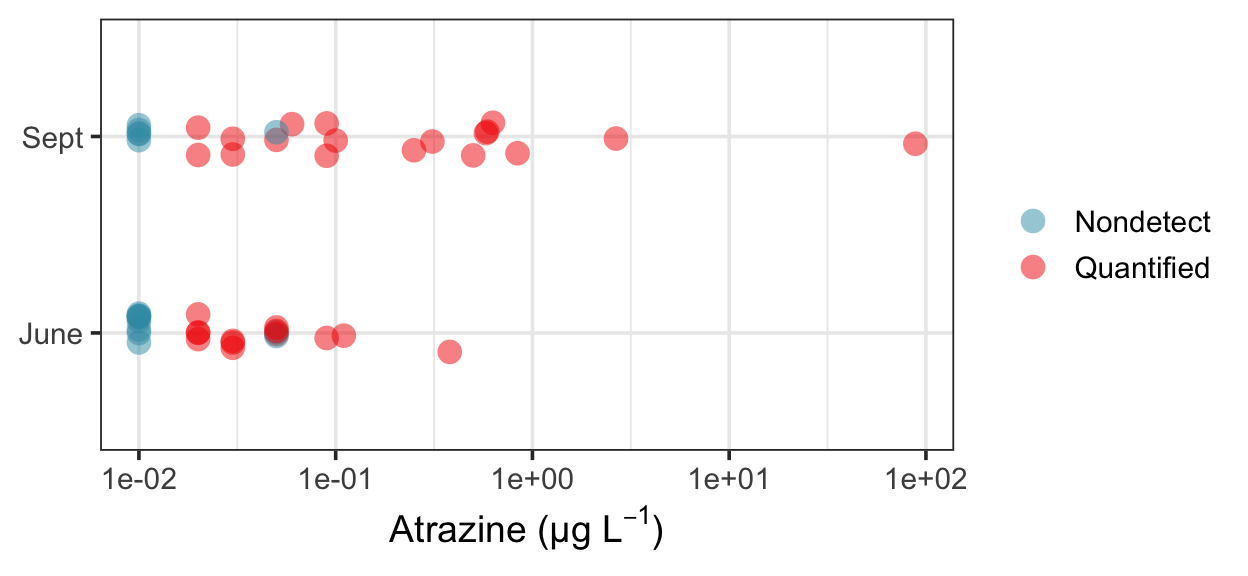
And here are the test results. These are close to the values in Helsel (2012), but not exactly the same. I suspect there are a few typos in the table, which may have something to do with it. For example, while most of the scores calculated by ppw_test() are consistent with those reported in the table, line 11, column 3 list a score of 0.55 for the second-highest value in column 1, while ppw_test() calculates a score of -0.54, much closer to the value of -0.67 corresponding to the largest value in column 1. There is a similar problem on line 12.

helsel %>% 
  mutate(
    june_cen = str_detect(june, "<"),
    sept_cen = str_detect(september, "<"),
  ) %>% 
  mutate_if(is.character, ~ as.numeric(str_remove(.x, "<"))) %>% 
  with(ppw_test(june, september, june_cen, sept_cen, "less"))

$statistic
[1] 3.012394

$p.value
[1] 0.001295979

Helsel, Dennis R. 2012. Statistics for Censored Environmental Data Using Minitab and R. 2nd ed. Wiley Series in Statistics in Practice. Hoboken, N.J: Wiley.

Lorenz, Dave. 2017. “SmwrQW–an R Package for Managing and Analyzing Water-Quality Data, Version 0.7.9.” Open File Report. U.S. Geological Survey.