Benjamin Trueman: Comparing water quality time series using a generalized additive mixed model

Ben Trueman

In a 2016 paper (Trueman and Gagnon 2016), I evaluated the effect of cast iron distribution mains on the lead concentrations due to lead pipes downstream from those mains. This question has relevance for minimizing lead in drinking water and for prioritizing lead pipe replacement; if a lead pipe is connected to an unlined iron distribution main, lead levels reaching the consumer are likely to be higher.

In the paper, I used the arima() function in R with a matrix of external regressors to account for the effect of the distribution main and autocorrelation in the time series of lead concentrations. But linear regression was only a rough approximation of the concentration time series’ behaviour, and I think using a generalized additive model would have been a better choice. Here, I revisit those data, using mgcv::gamm() to fit a generalized additive mixed model and nlme::corCAR1() to include a continuous time first-order autoregressive error structure.

First, I built the model, using s() to fit a separate smooth to each category of lead time series. (The categories are defined by the distribution main—PVC or cast iron—and the lead pipe configuration—full lead or half lead, half copper.) In this model, the smooths differ in their flexibility and shape (Pedersen et al. 2019). They are centered, so the grouping variables are added as main effects (see the documentation for mgcv::s()). I use tidyr::nest() to allow for list columns that include the model and predicted values along with the data.

fe_gam <- jdk_pl %>% 
  filter(fraction == "total") %>% 
  mutate_if(is.character, factor) %>% 
  mutate(lsl_grp = interaction(pipe_config, main)) %>% 
  arrange(fraction, lsl, time_d) %>% 
  group_by(fraction) %>% 
  nest() %>% 
  ungroup() %>% 
  mutate(
    model = map(
      data,
      ~ mgcv::gamm(
        log(pb_ppb) ~ s(time_d, by = lsl_grp) + main + pipe_config, # model I
        correlation = nlme::corCAR1(form = ~ time_d | lsl),
        method = "REML",
        data = .x
      )
    )
  )

Next, I predicted from the model over the range of x values, and constructed a pointwise (approximate) 95% confidence band using the standard errors of the fitted values.

fe_gam <- fe_gam %>% 
  mutate(
    preds = map2(
      model, data, 
      ~ predict(.x$gam, newdata = .y, se = TRUE)
    ),
    preds = map2(
      preds, model, 
      ~ tibble(fit = .x$fit, se_fit = .x$se.fit) %>% 
        mutate(
          lwr = fit - 2 * se_fit,
          upr = fit + 2 * se_fit,
          fit = fit
        ) %>% 
        mutate_at(vars(c(fit, lwr, upr)), exp)
    )
  )

Here are the data, the fitted model, and the confidence bands:

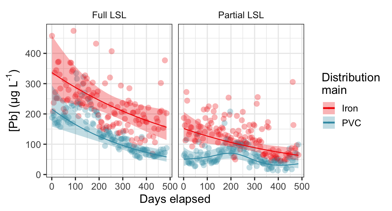
You’ll notice that some of the smooths—especially the Full LSL/PVC smooth—are smoother than the eye would expect. This is probably because the model is attributing some of the nonlinearity to autocorrelation, something discussed in more detail elsewhere (Simpson 2018).

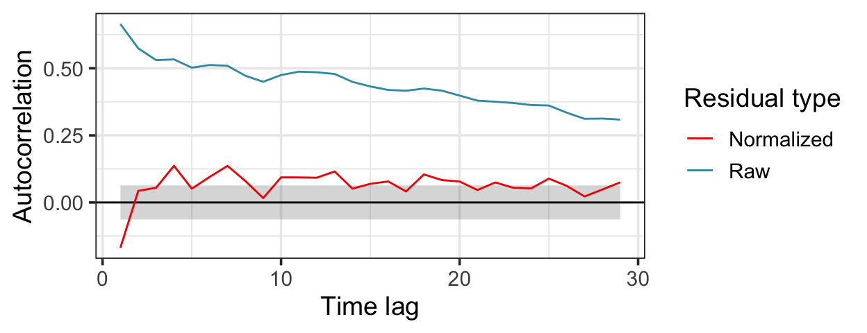
The model does a reasonably good job—but not a perfect job—accounting for autocorrelation in the time series. “Raw” and “normalized” residuals are defined in the help file to nlme::residuals.lme() under type. Essentially, raw residuals represent the difference between the observed and fitted values, while normalized residuals account for the estimated error structure. The grey shaded band in the figure below represents a 95% confidence interval on the autocorrelation of white Gaussian noise.

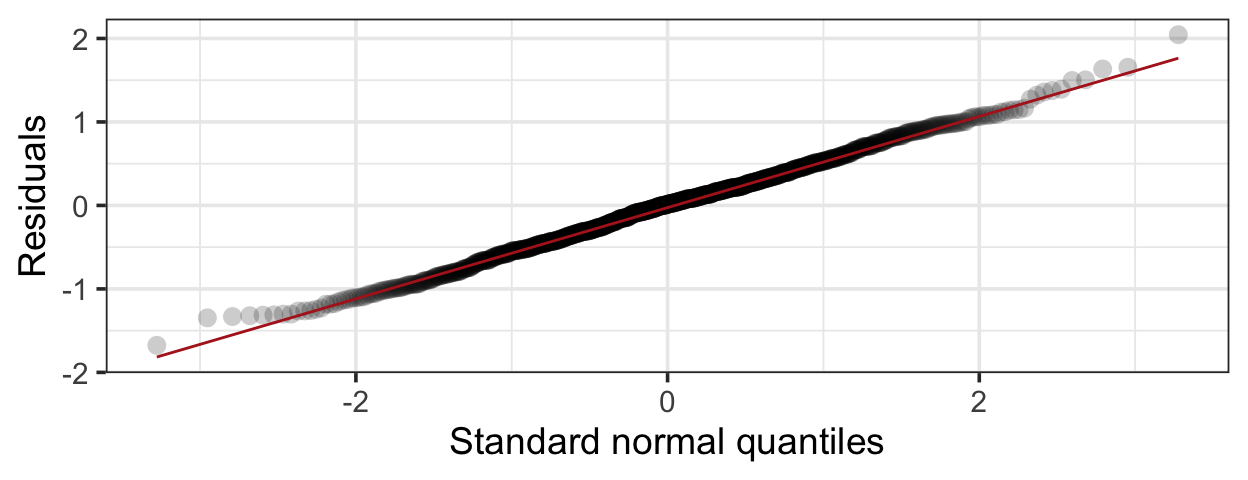
The natural log transformation yields a model with residuals that are approximately normal.

Finally, let’s have a look at the model summary. The effect of the distribution main is statistically significant, as is the effect of pipe configuration (which we’re less concerned about here). Based on the retransformed coefficient (exponentiating and subtracting one), the model estimates that lead release is 51% lower when the distribution main supplying the lead pipe is plastic as opposed to iron—an important result given the limited resources available to replace lead drinking water pipes.


Family: gaussian 
Link function: identity 

Formula:
log(pb_ppb) ~ s(time_d, by = lsl_grp) + main + pipe_config

Parametric coefficients:
                       Estimate Std. Error t value Pr(>|t|)    
(Intercept)             5.44408    0.07202  75.587   <2e-16 ***
mainpvc                -0.70833    0.08333  -8.501   <2e-16 ***
pipe_configpartial lsl -0.84626    0.08333 -10.156   <2e-16 ***
---
Signif. codes:  0 '***' 0.001 '**' 0.01 '*' 0.05 '.' 0.1 ' ' 1

Approximate significance of smooth terms:
                                    edf Ref.df      F p-value    
s(time_d):lsl_grpfull lsl.iron    1.000  1.000  7.718 0.00558 ** 
s(time_d):lsl_grppartial lsl.iron 1.000  1.000  9.904 0.00170 ** 
s(time_d):lsl_grpfull lsl.pvc     1.000  1.000 22.649   3e-06 ***
s(time_d):lsl_grppartial lsl.pvc  3.444  3.444  3.345 0.00880 ** 
---
Signif. codes:  0 '***' 0.001 '**' 0.01 '*' 0.05 '.' 0.1 ' ' 1

R-sq.(adj) =  0.564   
  Scale est. = 0.33246   n = 954

Pedersen, Eric J., David L. Miller, Gavin L. Simpson, and Noam Ross. 2019. “Hierarchical Generalized Additive Models in Ecology: An Introduction with Mgcv.” PeerJ 7 (May): e6876. https://doi.org/10.7717/peerj.6876.

Simpson, Gavin L. 2018. “Modelling Palaeoecological Time Series Using Generalised Additive Models.” Frontiers in Ecology and Evolution 6 (October): 149. https://doi.org/10.3389/fevo.2018.00149.

Trueman, Benjamin F., and Graham A. Gagnon. 2016. “Understanding the Role of Particulate Iron in Lead Release to Drinking Water.” Environmental Science & Technology 50 (17): 9053–60. https://doi.org/10.1021/acs.est.6b01153.

Comparing water quality time series using a generalized additive mixed model

References

Corrections

Citation