Diagnostics for censored autoregressive models fitted with brms

Posterior predictive checks and simulated residuals.

In a previous post (A brownification pause), I made an attempt at tackling a common problem in environmental science: analyzing autocorrelated time series with left-censored values (i.e., nondetects). As I’ve learned, one powerful tool for this type of problem is brms (Bürkner 2017, 2018), an R package for fitting Bayesian regression models via Stan (Stan Development Team 2021).

There are, however, relatively few tools that I’m aware of for posterior predictive checks of censored regression models. The R function bayesplot::ppc_km_overlay() is one, but it is only suitable for right-censored data, which are less common in environmental time series.

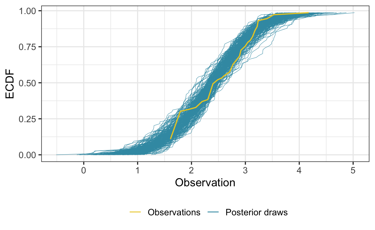
Here I use a similar approach to generate a posterior predictive check for a left-censored model. I use the R function NADA::cenfit() (Lee 2020) to estimate the empirical cumulative distribution function (ECDF) of the series and the posterior draws from the model. The function works by “flipping” the input—subtracting all values from a constant larger than any value—and estimating the ECDF according to the Kaplan-Meier method (for right-censored data).

The following generates ECDFs of the data and posterior predictions according to this method:

pp_ecdf <- function(model, newdata, yval, log_t = TRUE) {
  
  ecdf_data_in <- newdata %>% 
  # convert censoring indicator to logical:
  mutate(ci = ci == -1) %>% 
  filter(!is.na({{yval}}))
  
  ecdf_data <- NADA::cenfit(
    obs = if(log_t) {
      log(pull(ecdf_data_in, {{yval}}))
    } else {
      pull(ecdf_data_in, {{yval}})
    },
    censored = ecdf_data_in$ci
  )

ecdf_pp <- tidybayes::add_predicted_draws(
    newdata, 
    model,
    ndraws = 200
  ) %>% 
  ungroup() %>% 
  group_by(.draw) %>% 
  nest() %>% 
  ungroup() %>% 
  mutate(
    cenfit = map(data, 
      ~ with(.x, 
        NADA::cenfit(
          obs = .prediction, 
          censored = rep(FALSE, length(.prediction))
        )
      )
    ),
    cenfit_summ = map(cenfit, summary)
  ) %>% 
  unnest(cenfit_summ) %>% 
  select(where(~ !is.list(.x))) 

  bind_rows(
    "Posterior draws" = ecdf_pp,
    "Observations" = summary(ecdf_data),
    .id = "type"
  )
}

Here I’ve superimposed the ECDF of the time series on the ECDFs estimated using 200 draws from the posterior distribution of the brms::brm() model. From this plot, it appears that the posterior draws approximate the data reasonably well.

Another difficulty in evaluating models fitted to censored time series is residuals analysis. Here I adopt the approach of Wang and Chan (2018), generating simulated residuals by substituting censored and missing values of the time series with a draw from the posterior distribution of the fitted model and refitting the model on the augmented data. I then generated residual draws from the updated model.

The function below does the simulation:

simulate_residuals <- function(
  model, 
  newdata, 
  yval, 
  file, 
  seed = NULL,
  ...
) {
  
  data_aug <- tidybayes::add_predicted_draws(
    newdata,
    model,
    seed = seed,
    ndraws = 1
  ) %>% 
    ungroup() %>% 
    mutate(
      value = if_else(
        is.na({{yval}}) | ci == -1,
        .prediction,
        {{yval}}
      ),
      ci = 0 # no censoring
    ) %>%
    select(-starts_with("."))
  
  model_update <- update(
    model, 
    newdata = data_aug,
    file = file,
    cores = 4,
    seed = seed,
    ...
  )
  
  model_resids <- tidybayes::add_residual_draws(
    object = model_update,
    newdata = data_aug,
    method = "posterior_epred"
  )
  
  list(
    model = model_update, 
    residuals = model_resids, 
    data = data_aug
  )
  
}

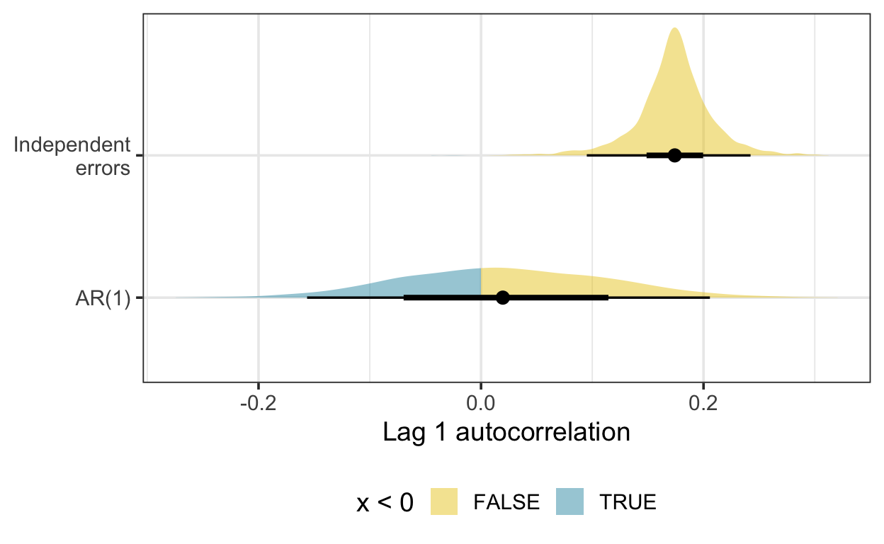
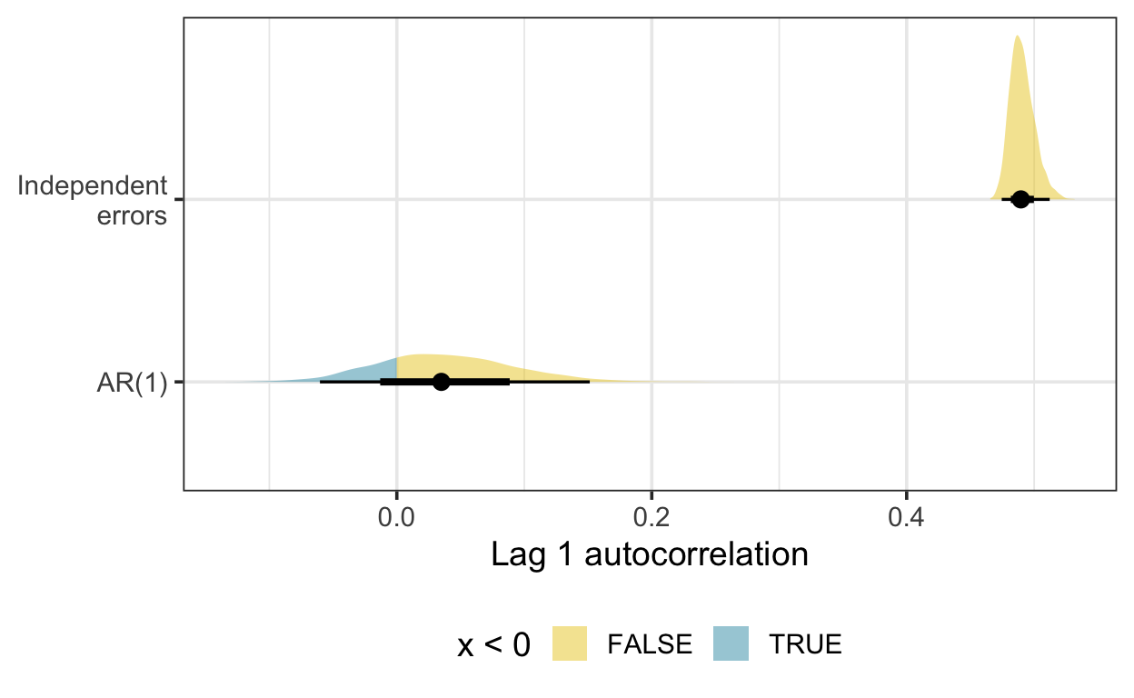
Here is the density of the lag one autocorrelation, estimated using residual draws from Bayesian GAMs fitted with and without a first-order autoregressive (AR(1)) term. There is some indication here that the GAM with an AR(1) term is accounting for residual autocorrelation.

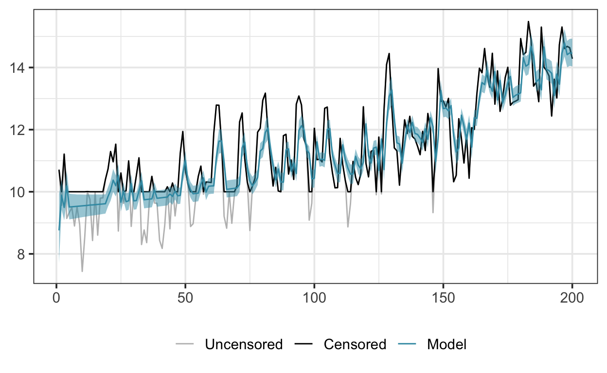
For a bit more verification, I fitted a similar GAM to a simulated dataset, generated by adding an AR(1) series to a nonlinear trend, as follows:

lcl <- 10 # lower censoring limit

simdat <- withr::with_seed(101, {
  tibble(
  x = 1:200,
  y_t = 1e-3 * x + 1e-4 * x ^ 2,
  e = arima.sim(list(ar = .5), length(y_t)) %>% 
    as.numeric(),
  y = y_t + e + 10,
  y_star = pmax(y, lcl),
  ci = if_else(y < lcl, -1, 0)
)
})

Again, I fitted the GAM—and the equivalent model without an AR(1) term—using brms:

model_simdat <- brm(
  bf(y_star | cens(ci) ~ s(x) + ar(time = x, p = 1)),
  data = simdat,
  seed = 124,
  # save the model:
  file = here::here("model_simdat"),
  cores = 4,
  control = list(adapt_delta = .99)
)

Here are the simulated data and the fitted model:

And here is the ECDF overlay described above:

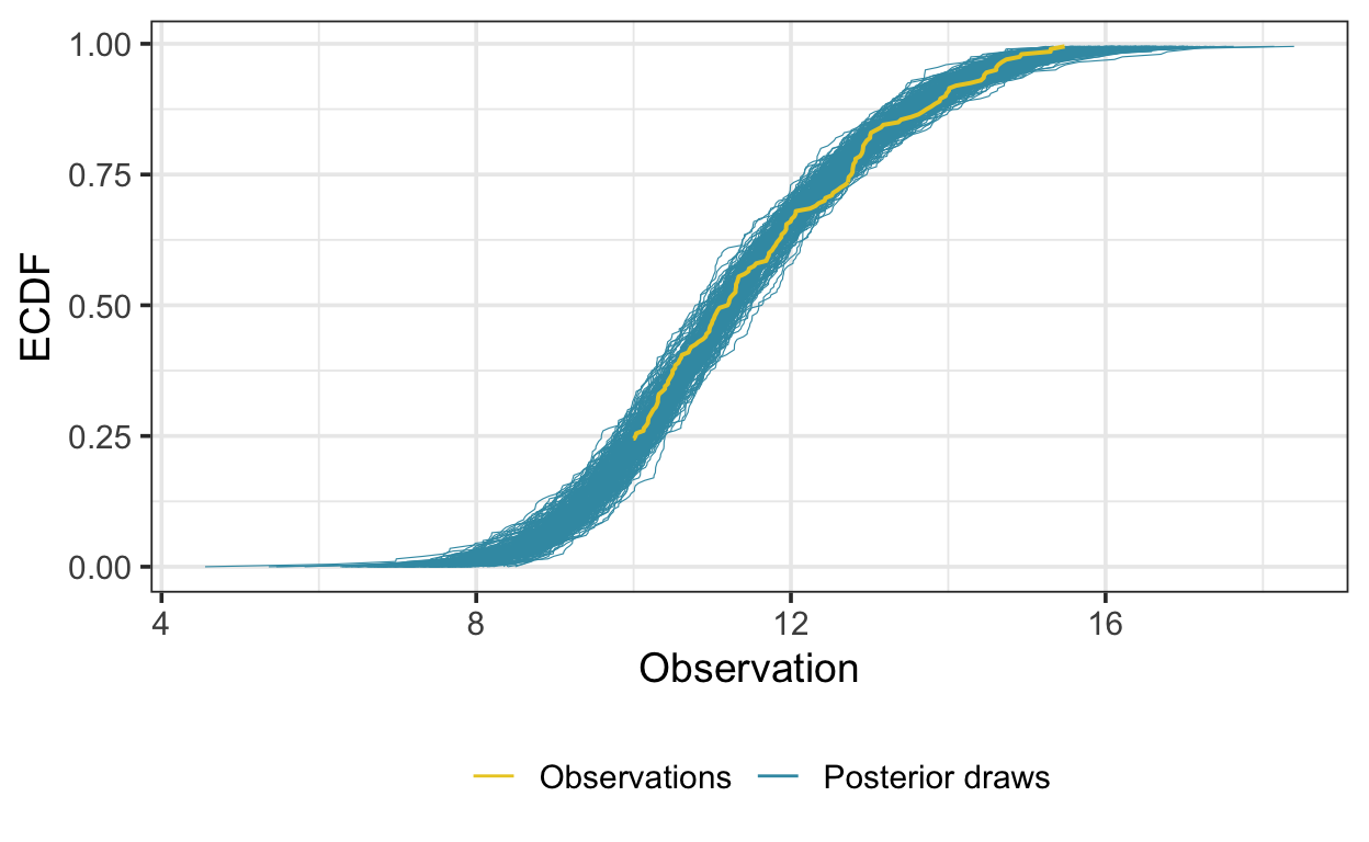
The first-order autocorrelation estimate from the simulated residuals suggests that the model is accounting for autocorrelation in the residuals, as expected:

And the estimate of the AR(1) term is 0.57, which is similar to true value of 0.5.