Building a continuous-time autoregressive model in brms

A simple modification of brms-generated Stan code to fit first-order autoregressive models to irregularly-spaced time series.

UPDATES:
1. This material is now implemented in an R package, bgamcar1, focused on GAMs with CAR(1) errors as a quick fix until a CAR(1) option is added to brms.
2. This post has been updated to reflect the changes to prior specification implemented in brms 2.17.0.

In recent posts, I’ve written about using brms to fit fully Bayesian autoregressive models to left-censored time series data. And while this approach is powerful, it is not easy to use for irregularly spaced series.

It turns out, though, that there is a straightforward generalization of the first-order autoregressive—AR(1)—model, called the continuous-time AR(1), or CAR(1). Whereas the AR(1) takes the form

\[x_t = \phi x_{t-1} + \epsilon_t\]

(where \(x\) is the time series, \(t\) is time, \(\phi\) defines the autocorrelation structure, and \(\epsilon_t\) is an independent error term), the CAR(1) model has the following autocorrelation structure:

\[h(s, \phi) = \phi^s, s\geq0, \phi\geq0 \] where \(s\) is a real number representing the time difference between successive observations. This model is implemented in R by the function nlme::corCAR1() (Pinheiro et al. 2021), and there is an open issue on GitHub discussing implementation in brms.

Not being able to wait for a future version of brms with CAR(1) as an option, I modified the brms generated Stan code to fit a CAR(1) model, as follows.

First, let’s simulate a couple of irregularly-spaced AR(1) processes:

stan_seed <- 1256

phi <- .75
p_ret <- .6 # proportion retained

withr::with_seed(stan_seed, {
  data <- tibble(
    x = 1:100,
    y1 = arima.sim(list(ar = phi), length(x)),
    y2 = arima.sim(list(ar = phi), length(x))
  ) %>% 
    pivot_longer(starts_with("y"), names_to = "g", values_to = "y")
  
  subset <- data %>% 
    slice_sample(prop = p_ret) %>% 
    arrange(g, x) %>% 
    group_by(g) %>% 
    mutate(
      x_lag = lag(x),
      d_x = replace_na(x - x_lag, 0) # spacing of observations
    ) %>% 
    ungroup()
})

Then, use brms to generate Stan code and the accompanying data as a list:

priors <- prior(normal(.5, .25), class = ar, lb = 0, ub = 1)
formula <- bf(y ~ ar(time = x, gr = g))

sdata <- brms::make_standata(formula, prior = priors, data = subset)
sdata$s <- subset$d_x # CAR(1) exponent 

scode <- brms::make_stancode(formula, prior = priors, data = subset)

Next, modify the Stan code to fit a CAR(1) model…

scode_car1 <- scode %>% 
  # add time difference variable s:
  str_replace(
    "response variable\\\n", 
    "response variable\n  vector[N] s;  // CAR(1) exponent\n"
  ) %>% 
  # set lower bound of zero on ar param:
  str_replace(
    "vector\\[Kar\\] ar;", 
    "vector<lower=0>[Kar] ar;"
  ) %>% 
  # convert AR process to CAR1:
  str_replace(
    "mu\\[n\\] \\+= Err\\[n, 1:Kar\\] \\* ar;", 
    "mu[n] += Err[n, 1] * pow(ar[1], s[n]); // CAR(1)"
  ) 

class(scode_car1) <- "brmsmodel"

… and pass the data list and the modified Stan code to rstan::stan() to fit the model.

stanfit <- rstan::stan(
  model_code = scode_car1,
  data = sdata,
  sample_file = "carmodel", # output in csv format
  seed = stan_seed
)

Once the chains have finished running, feed the Stan model back into brms, and have a look at the output of summary(). There are no obvious problems with convergence, given the lack of warnings from Stan and the \(\widehat{r}\) values being very close to 1.

fit <- brm(formula, data = subset, empty = TRUE)
fit$fit <- stanfit
fit <- rename_pars(fit)
summary(fit)

 Family: gaussian 
  Links: mu = identity; sigma = identity 
Formula: y ~ ar(time = x, gr = g) 
   Data: subset (Number of observations: 120) 
  Draws: 4 chains, each with iter = 2000; warmup = 1000; thin = 1;
         total post-warmup draws = 4000

Correlation Structures:
      Estimate Est.Error l-95% CI u-95% CI Rhat Bulk_ESS Tail_ESS
ar[1]     0.71      0.07     0.57     0.83 1.00     3547     2922

Population-Level Effects: 
          Estimate Est.Error l-95% CI u-95% CI Rhat Bulk_ESS Tail_ESS
Intercept    -0.20      0.25    -0.67     0.30 1.00     3045     2351

Family Specific Parameters: 
      Estimate Est.Error l-95% CI u-95% CI Rhat Bulk_ESS Tail_ESS
sigma     1.17      0.08     1.03     1.33 1.00     3573     2603

Draws were sampled using (). For each parameter, Bulk_ESS
and Tail_ESS are effective sample size measures, and Rhat is the potential
scale reduction factor on split chains (at convergence, Rhat = 1).

Since the brmsfit object doesn’t contain the CAR(1) formula, a few extra steps are needed to generate predictions. First, we generate draws from the model without the autocorrelation structure, then we apply a CAR(1) filter to the data, and then we summarize the filtered draws using median_qi(). Plot the medians along with the data, adding the 0.025 and 0.975 quantiles as a ribbon:

# extract AR(1) draws:
phi <- as_draws_df(fit, "ar[1]") %>% 
  as_tibble()

# generate draws from the model without the autocorrelation structure:
pred_car1 <- tidybayes::add_epred_draws(subset, fit, incl_autocor = FALSE) %>% 
  ungroup() %>% 
  select(-c(.chain, .iteration)) %>% 
  arrange(.draw, g, x) %>% 
  left_join(phi, by = ".draw") %>% 
  # add the CAR(1) structure:
  group_by(.draw, g) %>% 
  mutate(
    r_lag = replace_na(lag(y - .epred), 0),
    .epred = .epred + r_lag * `ar[1]` ^ d_x
  ) %>% 
  ungroup() %>% 
  # summarize:
  select(-c(r_lag, `ar[1]`)) %>% 
  group_by(across(matches(paste(names(subset), collapse = "|")))) %>% 
  ggdist::median_qi() %>% 
  ungroup()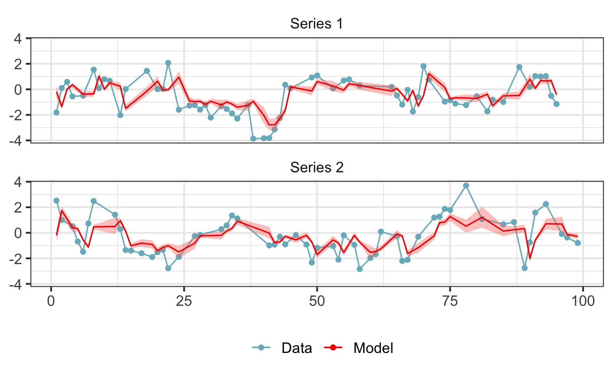

And that’s it! The model recovers the parameters used to generate the simulated data well in this case—the mean of the posterior of \(\phi\) is 0.71—which is a good sign that we’re on the right track.