Regression models with censored predictors

Another modification of brms-generated Stan code, this time to fit regression models with censored predictors.

Recently, I’ve encountered several regression problems where the predictors are partially censored. To tackle this issue, I turned to Paul Bürkner’s excellent package for Bayesian regression, brms (Bürkner 2017). Paul has written a helpful vignette on handling missing values. The general strategy we’ll use here is outlined in that vignette: imputation during model fitting by declaring the missing values as parameters. That is, we’ll fit a multivariate model that imputes missing values in both the predictor and the response variable. The only problem is that brms doesn’t handle censored predictors, so we’ll need to customize our approach a little bit.

Let’s start by loading the following packages:

library("tidyverse")
library("glue")
library("ggdist")
library("withr")
library("brms")
library("rstan")
options(mc.cores = parallel::detectCores()) # for parallel MCMC chains

Then we’ll need to simulate some data:

n <- 50 # total number of observations
lcl <- -1 # lower censoring limit

with_seed(1235, {
  data <- tibble(
    x = rnorm(n, 0, 2),
    y = 2 * x + rnorm(n)
  )
})

data$x_star <- data$x
data$x_star[c(3, 29)] <- NA # add missing values
data$cens_x_star <- replace_na(data$x_star < lcl, FALSE) # censoring indicator
data$x_star <- pmax(data$x_star, lcl) # left-censor values

# train/test split:
train <- 1:25 
data_train <- data[train, ]
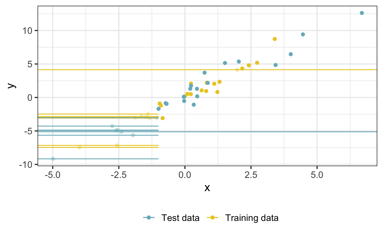
data_test <- data[-train, ]

Let’s plot the simulated data so we can see what we’re dealing with. Missing x values are shown as horizontal lines, and left-censored x values are shown as horizontal line segments extending from the left edge of the plot to the censoring limit of -1. The true values corresponding to the censored and missing observations are transparent.

The trick at this point is to treat left-censored x values as missing values with an upper bound equal to the censoring limit, as described in the Stan manual. But since brms doesn’t do this we’ll have to code it ourselves. We’ll need two functions: one to modify the data list and another to modify the code that brms passes to Stan:

modify_standata <- function(sdata, data, lcl, var) {
  
  if (length(lcl) != length(var)) stop("lengths of 'var' and 'lcl' must be equal")
  
  varstan <- str_remove_all(var, "_")
  
  for(i in seq_len(length(var))) {
    sdata[[paste0("Ncens_", varstan[i])]] <- sum(data[[paste0("cens_", var[i])]]) # number of left-censored
    # positions of left-censored:
    sdata[[paste0("Jcens_", varstan[i])]] <- as.array(seq_len(nrow(data))[data[[paste0("cens_", var[i])]]]) 
    sdata[[paste0("U_", varstan[i])]] <- lcl[i] # left-censoring limit
  }
  
  sdata
}

modify_stancode <- function(scode, var) {
  
  var <- str_remove_all(var, "_")
  
  for(i in seq_len(length(var))) {
    
    # modifications to data block:
    n_cens <- glue("int<lower=0> Ncens_{var[i]};  // number of left-censored")
    j_cens <- glue("int<lower=1> Jcens_{var[i]}[Ncens_{var[i]}];  // positions of left-censored")
    u <- glue("real U_{var[i]};  // left-censoring limit")
    # modifications to parameters block:
    y_cens <- glue("vector<upper=U_{var[i]}>[Ncens_{var[i]}] Ycens_{var[i]};  // estimated left-censored")
    # modifications to model block:
    yl <- glue("Yl_{var[i]}[Jcens_{var[i]}] = Ycens_{var[i]}; // add imputed left-censored values")
    
    scode <- scode %>%
      # modifications to data block:
      str_replace(
        "(data \\{\n(.|\n)*?)(?=\n\\})",
        paste(c("\\1", n_cens, j_cens, u), collapse = "\n  ")
      ) %>% 
      # modifications to parameters block:
      str_replace(
        "(parameters \\{\n(.|\n)*?)(?=\n\\})",
        paste(c("\\1\n  ", y_cens), collapse = "")
      ) %>% 
      # modifications to model block:
      str_replace(
        "(model \\{\n(.|\n)*?)(?=\n    mu_)",
        paste(c("\\1\n    ", yl), collapse = "")
      )
    
  }
  
  class(scode) <- "brmsmodel"
  
  scode
    
}

We’ll also need a function to impute missing and censored values for prediction using the fitted model:

impute <- function(data, model, var, mi = NULL, cens = NULL, id = NULL) {
  
  varstan <- str_remove_all(var, "_")
  
  censored <- as_draws_df(model) %>% 
    as_tibble() %>% 
    select(starts_with(paste0("Ycens_", varstan))) %>% 
    t()
  
  if (!is.null(id)) {
    censored <- censored[id, ]
  }
  
  missing <- as_draws_df(model) %>% 
    as_tibble() %>% 
    select(starts_with(paste0("Ymi_", varstan))) %>% 
    t()
  
  ndraws <- ncol(censored)
  
  map(
    seq_len(ndraws),
    \(x) {
      data_imputed <- data
      if (!is.null(mi)) {data_imputed[mi, var] <- missing[, x]}
      if (!is.null(cens)) {data_imputed[cens, var] <- censored[, x]}
      data_imputed
    }, .progress = TRUE
  )
  
}

Now we’re ready to set up and run the model. First we need a formula that defines a model for both y and x. Since we don’t have anything else to go on, the model for x is intercept only, but we should be able to do better than that in many real applications. The calls to mi() define missing values and how they’re handled during model fitting—see the brms vignette for details.

bform <- bf(y | mi() ~ mi(x_star)) + 
  bf(x_star | mi() ~ 1) +
  set_rescor(FALSE)

Next, we modify the data and code passed to Stan…

sdata <- make_standata(bform, data = data_train) %>% 
  modify_standata(data_train, lcl, "x_star")
scode <- make_stancode(bform, data = data_train) %>% 
  modify_stancode("x_star")

… and fit (and save) the model using rstan::stan.

stanseed <- 1257
model_rstan <- stan(
  model_code = scode,
  data = sdata,
  sample_file = "model-censored-x", # save model as CSVs
  seed = stanseed
)

We can load the fitted model later using the following:

model_rstan <- read_stan_csv(list.files(pattern = "model-censored-x_"))

Now we can generate posterior predictions along a regular sequence of predictor values, using the posterior draws for the slope and intercept:

post_draws <- as_draws_df(model_rstan) # posterior draws:

xnew <- seq(min(data$x), max(data$x), length.out = 25) # regular sequence of x-values

post_imp <- map(
  seq_len(nrow(post_draws)),
  ~ xnew * post_draws$`bsp_y[1]`[.x] + post_draws$Intercept_y[.x]
) %>%
  do.call(rbind, .)

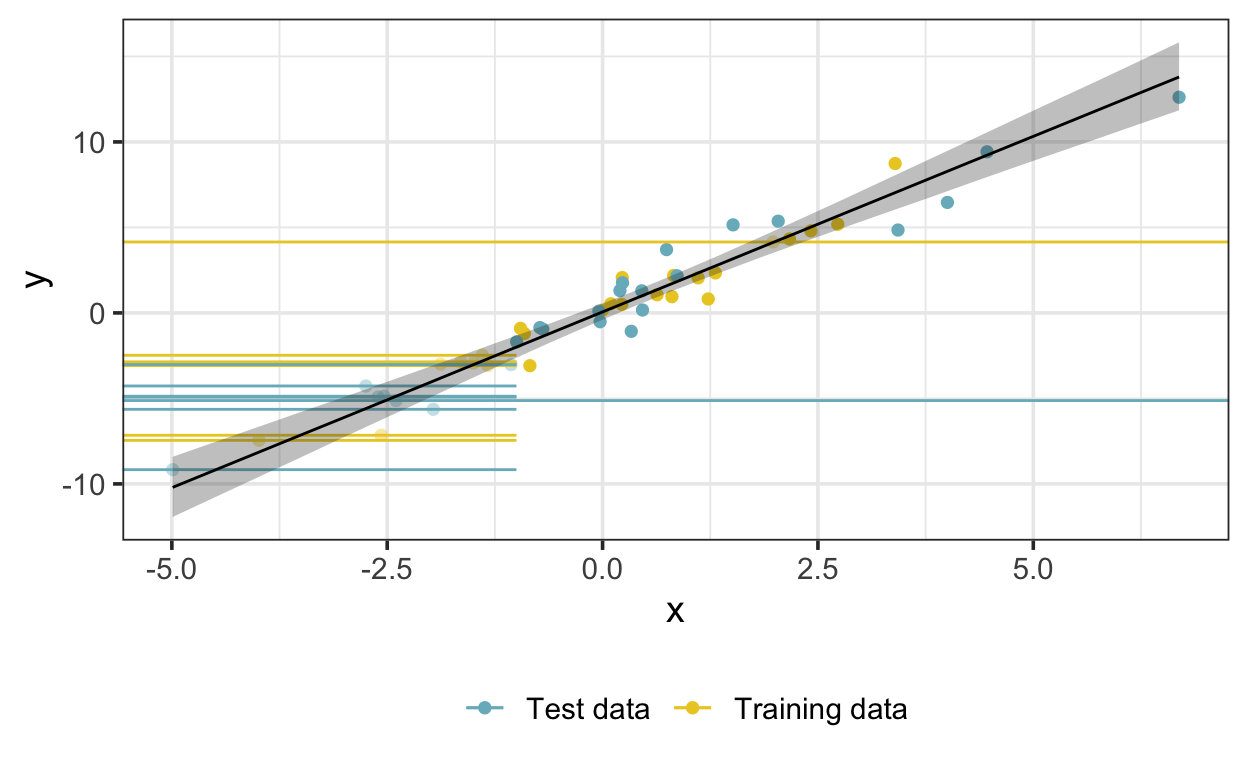
Here is the fitted model—the shaded region represents a 95% credible interval on the posterior expectation.

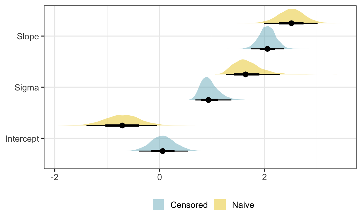
Let’s compare the parameter estimates from this model with those of a simple linear regression model that doesn’t account for censoring or missingness:

model_naive <- brm(
  y ~ x_star,
  data = data_train,
  file = "model-naive",
  file_refit = "on_change"
)
post_draws_naive <- as_draws_df(model_naive)

The posterior draws of the censoring model match the true parameter values closely, while those of the naive model are a poor match:

To estimate prediction performance for the training data, we first impute the censored and missing values. This generates a list of imputed datasets as long as the number of posterior samples.

data_train_imputed <- impute(data_train, model_rstan, "x_star", sdata$Jmi_xstar, sdata$Jcens_xstar)

Then, we can calculate RMSE for the training data by generating predictions using the imputed datasets and the posterior draws of the model parameters:

rmse <- function(y, yhat) {
  sqrt(mean((y - yhat) ^ 2))
}
rmse_train <- map2_dbl(
  seq_len(nrow(post_draws)),
  data_train_imputed,
  \(x, y) {
    yhat <- y$x_star * post_draws$`bsp_y[1]`[x] + post_draws$Intercept_y[x]
    rmse(y$y, yhat)
  }
)
median_qi(rmse_train) # summarize

          y      ymin     ymax .width .point .interval
1 0.8905452 0.7783883 1.154363   0.95 median        qi

We can also estimate out-of-sample error by imputing missing values and generating posterior predictions. Imputing censored values in the test data, though, is slightly more complicated: since there is no guarantee that model predictions will fall below the censoring limit, we impute by refitting the model to the training set, augmented by the censored observations from the test set:

data_combined <- bind_rows(data_train, data_test[data_test$cens_x_star, c("x_star", "cens_x_star")])
sdata_combined <- make_standata(bform, data = data_combined) %>% 
  modify_standata(data_combined, lcl, "x_star")

We fit the same model as we did on the training data. The augmented model excludes all of the response values from the test set, though: these are imputed during model fitting but not used further.

model_rstan_combined <- stan(
  model_code = scode,
  data = sdata_combined,
  sample_file = "model-censored-x-combined",
  seed = stanseed,
  control = list(adapt_delta = .99)
)

After fitting, we impute the censored values, and fill in the missings by posterior prediction.

data_test_imputed <- impute(
  data = data_test,
  model = model_rstan_combined,
  var = "x_star",
  mi = NULL,
  cens = seq_len(nrow(data_test))[data_test$cens_x_star],
  id = 8:13
) %>% 
  # impute missings via posterior prediction:
  map2(
    seq_len(nrow(post_draws)),
    ~ .x %>% 
        mutate(
          x_star = if_else(
            is.na(x_star), 
            post_draws$Intercept_xstar[.y], 
            x_star
          )
        )
  )

Then, we generate test predictions…

preds_test <- map2(
  seq_len(nrow(post_draws)),
  data_test_imputed,
  ~ .y$x_star * post_draws$`bsp_y[1]`[.x] + post_draws$Intercept_y[.x]
)

… and use them to calculate the RMSE. Since the naive model uses complete cases only, we omit the row with a missing x value from the RMSE calculation for the censored model.

rmse_test <- apply(
  do.call(rbind, preds_test)[,-4], 
  1, 
  \(x) rmse(x, data_test$y[-4])
) %>% 
  median_qi()

rmse_naive <- apply(
  posterior_epred(model_naive, newdata = data_test)[ , -4],
  1,
  \(x) rmse(x, data_test$y[-4])
) %>% 
  median_qi()

Finally, let’s compare the predictions:

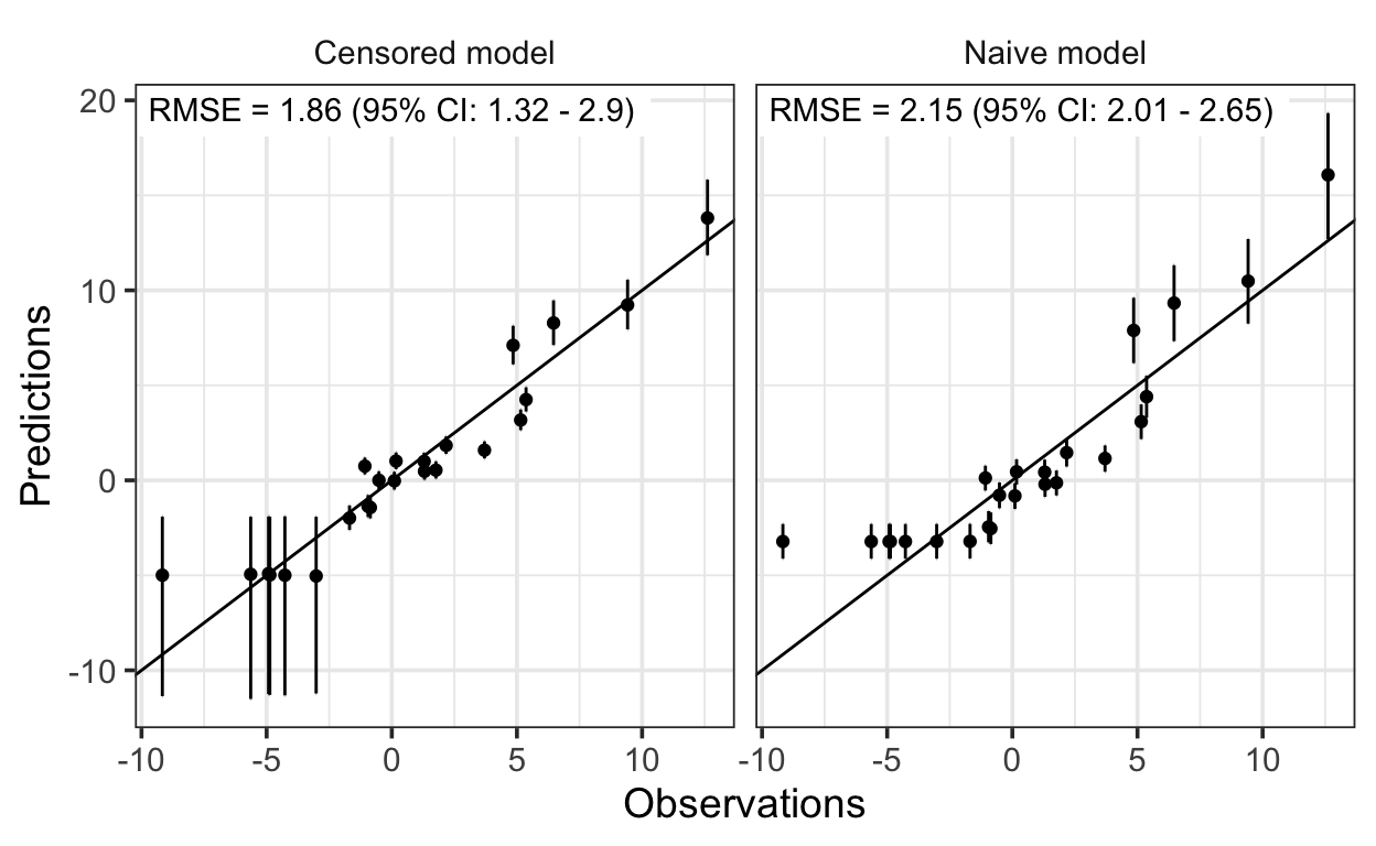
And that’s it! The linear regression model with censored predictors recovers the true parameter values well and yields better prediction performance than the simple linear regression model.