Probabilistic principal component analysis for censored data

Application of Bayesian PCA to a heavily left-censored (simulated) dataset.

Principal component analysis (PCA) has been a recent focus in my efforts to find Bayesian versions of statistical methods that play nicely with censored data. The solution in this case is probabilistic PCA (Bishop 1998), demonstrated here using a simulated dataset and then fitted using Stan via the R interface cmdstanr. The simulation approach and Stan program borrow heavily from this Jupyter notebook—I (roughly) translate the Python to R and modify the simulation and Stan program to allow imputation of censored values as a step in the model fitting process.

Probabilistic PCA is a latent variable model that can be written as follows:

\[ y \sim N(Wz, \sigma^2I) \\ z \sim N(0, I) \] where \(y\) is an \(n \times d\) matrix of data, \(z\) is an \(n \times k\) matrix of latent variables with \(k \leq d\), \(W\) is a \(d \times k\) transformation matrix mapping from the latent space to the data space, and \(\sigma^2\) is the error variance.

To explore this model, we’ll need the following packages:

library("tidyverse")
library("here")
library("cmdstanr")
library("MASS", include.only = "mvrnorm")
library("pracma", include.only = "orth")
library("withr")

First, we need to simulate from the data-generating process:

n <- 500 # number of observations
d <- 2 # number of data dimensions
k <- 1 # number of latent space dimensions
sigma2 <- 0.05 # error variance

with_seed(124563, {
  # sample latent variable Z:
  Z <- mvrnorm(n, mu = rep(0, k), Sigma = diag(1, k, k)) # n x k
  # create orthogonal transformation matrix:
  W <- orth(matrix(runif(d * k), d, k)) # d x k
  # generate additive noise:
  noise <- mvrnorm(n, mu = rep(0, d), Sigma = sigma2 * diag(1, d, d)) # n x d
})

# generate data:
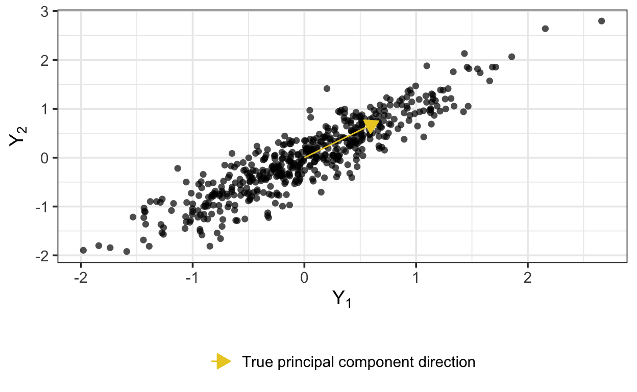
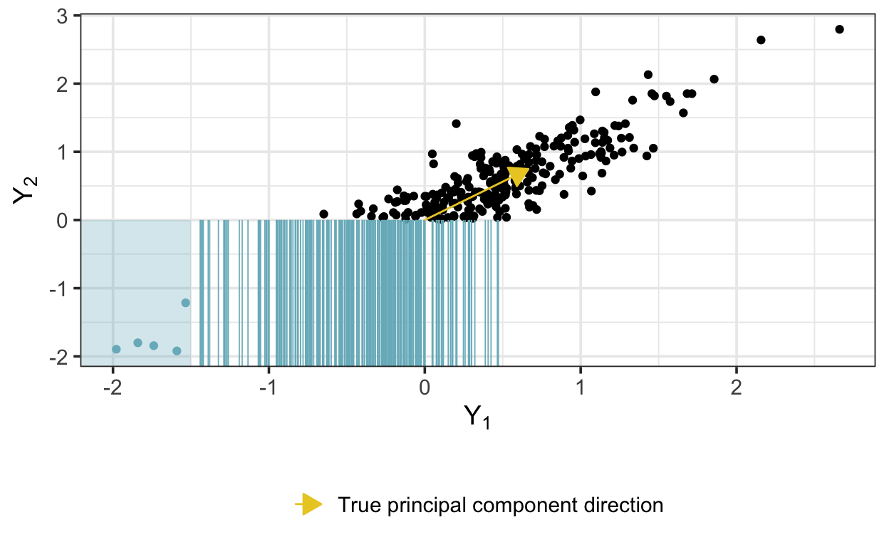
Y <- W %*% t(Z) + t(noise)

Here are the data, along with the first principal component—that is, the first and only column of \(W\).

Next, we’ll need to put the data into a list for passing to cmdstanr methods.

standata <- list(
  N = n,
  D = d,
  K = k,
  y = Y
)
stanseed <- 215678

Read the Stan program and compile (the Stan code is available in the Jupyter notebook linked at the top of this post; I’ve modified the basic version only slightly).

ppca_scode <- readLines(here("ppca.stan"))
model <- cmdstan_model(stan_file = write_stan_file(ppca_scode))

Once compiling is done, sample from the posterior:

fit <- model$sample(data = standata, seed = stanseed, parallel_chains = 4)
fit$save_output_files(
  dir = "models", basename = "ppca", random = FALSE, timestamp = FALSE
)

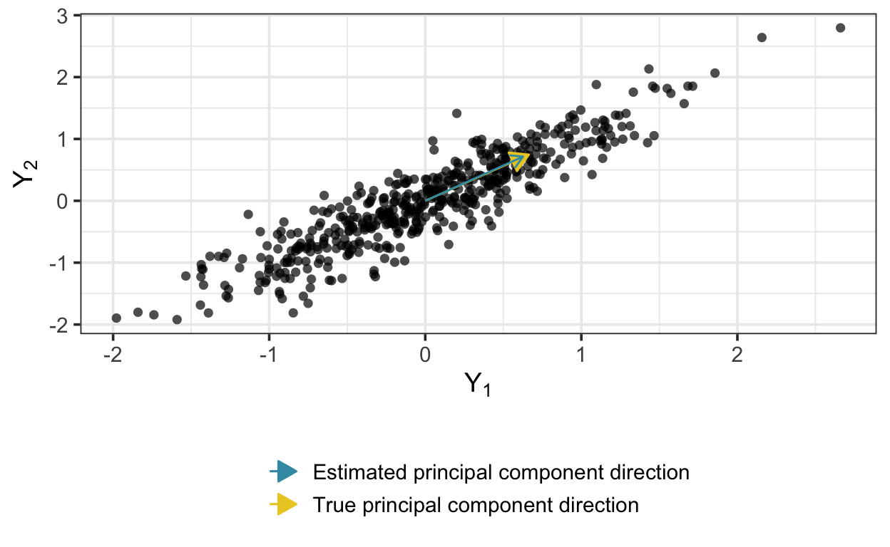
The model recovers the transformation matrix quite well:

# extract draws:
draws_df <- fit$draws(format = "df")

# extract the raw transformation matrix:
A <- draws_df %>% 
  select(starts_with("A"))

# calculate the posterior mean and orthogonalize:
W_est <- A %>% 
  apply(2, \(x) mean(abs(x))) %>% 
  matrix(standata$D, standata$K) %>% 
  orth()

Same goes for the error variance:

mean(draws_df$sigma ^ 2)

[1] 0.04871603

To compare the latent variable estimates with the true values, we have to correct for the sign of \(W\), iteration-by-iteration:

# extract the signs of transformation matrix:
S <- tibble(sign = apply(sign(A), 1, unique)) 
# extract raw latent variables:
X <- draws_df %>% 
  select(starts_with("x"))
# sign correction:
Z_est <- X %>% 
  apply(2, \(x) x * S$sign) %>% 
  apply(2, mean) %>% 
  matrix(standata$N, standata$K) %>% 
  `colnames<-`(paste0("pc", seq_len(standata$K))) %>% 
  as_tibble()

Here are the posterior means of the latent variables compared with the true \(z\):

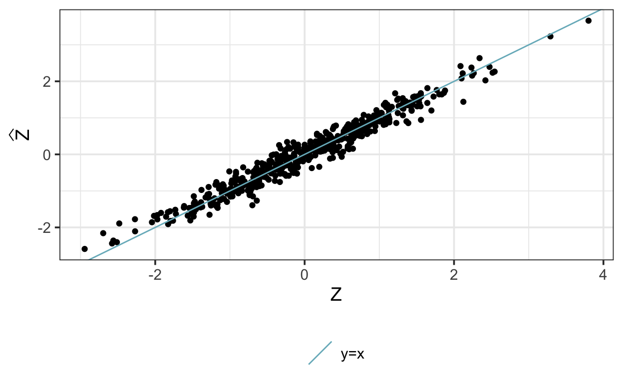
This is very similar to the PCA solution:

pca <- princomp(t(Y))
pca$loadings[,1] # principal component directions

[1] 0.6589110 0.7522209

W_est[,1] # transformation matrix

[1] 0.6591170 0.7520404

# correlation between PC scores and latent variable:
cor(Z_est, pca$scores[,1])

         [,1]
pc1 0.9999959

Now let’s turn to the problem of censoring. First, let’s modify the simulated data to introduce left-censoring:

# set censoring limits:
lcl_1 <- -1.5 # left-censoring limit, y1
lcl_2 <- 0 # left-censoring limit, y2

# simulate left-censored data:
Y_cens <- Y
Y_cens[1, ] <- pmax(Y[1, ], lcl_1)
Y_cens[2, ] <- pmax(Y[2, ], lcl_2)

# censored indicators:
nondetect_1 <- Y[1,] < lcl_1
nondetect_2 <- Y[2,] < lcl_2

Values censored in one dimension are represented as blue lines and values censored in both dimensions are represented as points within the shaded region:

We’ll need a new list of data inputs to pass to cmdstan functions:

standata_cens <- list(
  N = n,
  D = d,
  K = k,
  y = Y_cens,
  Ncens_y1 = sum(nondetect_1),
  Ncens_y2 = sum(nondetect_2),
  Jcens_y1 = seq_len(n)[nondetect_1],
  Jcens_y2 = seq_len(n)[nondetect_2],
  U_y1 = lcl_1,
  U_y2 = lcl_2
)

The following Stan program estimates the latent variable model after imputing censored data:

// modified from: https://github.com/nbip/PPCA-Stan/blob/master/PPCA.ipynb

data {
  int<lower=1> N; // num datapoints
  int<lower=1> D; // num data-space dimensions
  int<lower=1> K; // num latent space dimensions
  array[D, N] real y;
  // data for censored imputation:
  int<lower=0> Ncens_y1; // number of censored, y1
  int<lower=0> Ncens_y2; // number of censored, y2
  array[Ncens_y1] int<lower=1> Jcens_y1; // positions of censored, y1
  array[Ncens_y2] int<lower=1> Jcens_y2; // positions of censored, y2
  real U_y1; // left-censoring limit, y1
  real U_y2; // left-censoring limit, y2
}
transformed data {
  matrix[K, K] Sigma; // identity matrix
  vector<lower=0>[K] diag_elem;
  vector<lower=0>[K] zr_vec; // zero vector
  for (k in 1 : K) {
    zr_vec[k] = 0;
  }
  for (k in 1 : K) {
    diag_elem[k] = 1;
  }
  Sigma = diag_matrix(diag_elem);
}
parameters {
  matrix[D, K] A; // transformation matrix / PC loadings
  array[N] vector[K] x; // latent variables
  real<lower=0> sigma; // noise variance
  // censored value parameters:
  array[Ncens_y1] real<upper=U_y1> Ycens_y1; // estimated censored, y1
  array[Ncens_y2] real<upper=U_y2> Ycens_y2; // estimated censored, y2
}
transformed parameters {
  // combine observed with estimated censored:
  array[D, N] real yl = y;
  yl[1, Jcens_y1] = Ycens_y1;
  yl[2, Jcens_y2] = Ycens_y2;
}
model {
  for (i in 1 : N) {
    x[i] ~ multi_normal(zr_vec, Sigma);
  } // zero-mean, identity matrix
  for (i in 1 : N) {
    for (d in 1 : D) {
      //y[d,i] ~ normal(dot_product(row(A, d), x[i]), sigma);
      target += normal_lpdf(yl[d, i] | dot_product(row(A, d), x[i]), sigma);
    }
  }
}
generated quantities {
  vector[N] log_lik;
  for (n in 1 : N) {
    for (d in 1 : D) {
      log_lik[n] = normal_lpdf(yl[d, n] | dot_product(row(A, d), x[n]), sigma);
    }
  }
}

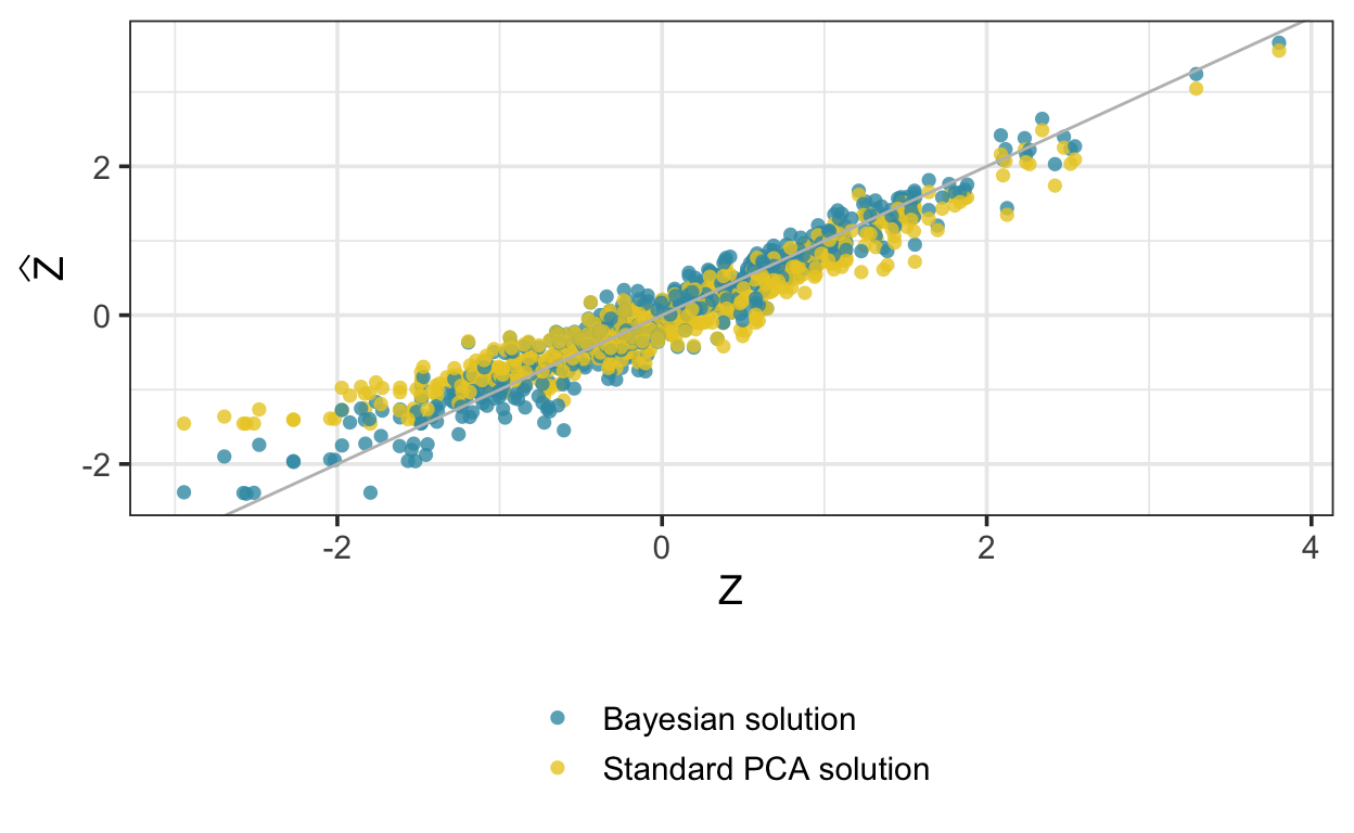
As above, we sample and extract the components. This time, the PCA solution is quite biased, while the Bayesian implementation does much better:

pca_cens <- princomp(t(Y_cens))
pca_cens$loadings[,1] # PCA solution

[1] 0.8476363 0.5305778

W_est_cens[,1] # Bayesian solution

[1] 0.6601378 0.7511445

W[,1] # true W

[1] 0.6646687 0.7471383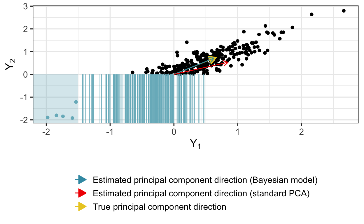

Here are the posterior means of the latent variables compared with the true \(z\); again, there is bias at the low end of the conventional principal component scores, but not with the Bayesian version.